The one pandas internal I teach all my new colleagues: the BlockManager
·When new members join our team, they usually are already fluent in data analysis with pandas and know their way around the typical quirks.
They know that they should use vectorised functions where possible and avoid using apply with a slow Python callable.
There are two main reasons, I teach them the BlockManager quite at the beginning.
The first reason is that it is actually a core architectural component that is neither visible from the API nor is it part of the most tutorials through which people learn pandas.
The other reason is that it has an impact on performance that is neither obvious from the code you were using nor that it always have the same (constant) impact on performance.
Even after writing this post, I cannot reliably tell you the performance of a simple df.loc[0:10, 'column'] = 1, my answer will be a “it depends!”.
The post here was written with the code base of pandas 1.0.x, it may not apply to newer versions.
What is the BlockManager?
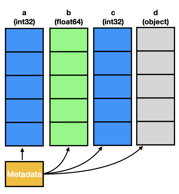
The typical perception about the structure of a pandas.DataFrame in memory is that there is a tiny bit of metadata and otherwise each column is stored as individual numpy.ndarray, pictured as follows.
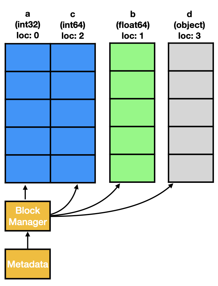
The actual memory layout of a DataFrame is a bit different though (see the figure below).
This is due to the fact that the data structure is not simply a dict of arrays.
Instead a pandas.DataFrame is a combination of an index (omitted in the image) and the data stored in blocks as managed by the BlockManager.
Wes McKinney introduced it in July 2011 as part of a general update on pandas development detailing the motivation and structure of the BlockManager.
For other explanatory visualisations about the internal structure of a DataFrame, have a look at the “pandas under the hood” presentation by Jeffrey Tratner.
The task of the BlockManager can be described very briefly through:
The BlockManager keeps columns of the exact same dtype in a single continuous memory region.
This one sentence typically is enough to convey what the BlockManager is doing in the background.
It helps to understand that some operations that seem constant in their runtime might be actually relative to the size of your DataFrame or a subset of it.
An important detail is also that columns are blocked by their data type. Columns that wouldn’t be neighbours by their actual position still land in the same block. This means a block also needs to store the position of its columns in the DataFrame.
To better understand what is happening, we look under the hood of a simple DataFrame.
# Create a DataFrame with two int64, two float64 and one int32 column.

import pandas as pd
import numpy as np

df = pd.DataFrame({
    'int64_1': np.array([1, 2, 3], dtype=np.int64),
    'int64_2': np.array([10, 20, 30], dtype=np.int64),
    'int32_1': np.array([9, 8, 7], dtype=np.int32),
    'float64_1': np.array([.1, .5, .7], dtype=np.float64)
})
This leaves us with the following table:
| int64_1 | int64_2 | int32_1 | float64_1 | |
|---|---|---|---|---|
| 0 | 1 | 10 | 9 | 0.1 |
| 1 | 2 | 20 | 8 | 0.5 |
| 2 | 3 | 30 | 7 | 0.7 |
With the previous explanation, the two columns int64_1 and int64_2 should be stored in the same block, i.e. the same numpy.ndarray.
Looking individually at the backing numpy.ndarray instances, they look like two distinct objects:
df['int64_1'].values
# > array([1, 2, 3])
type(df['int64_1'].values)
# > numpy.ndarray
df['int64_1'].values.shape
# > (3,)
df['int64_2'].values
# > array([10, 20, 30])
type(df['int64_2'].values)
# > numpy.ndarray
df['int64_2'].values.shape
# > (3,)
Instead of being separate objects, they are only views to the same base.
df['int64_1'].values.base
# > array([[ 1,  2,  3],
# >       [10, 20, 30]])

# As there is only one int32 array, its base is equal to the column values
df['int32_1'].values.base
# > array([[9, 8, 7]], dtype=int32)
To find how the DataFrame is stored in memory, we can look at its internal storage object df._data:
BlockManager
Items: Index(['int64_1', 'int64_2', 'int32_1', 'float64_1'], dtype='object')
Axis 1: RangeIndex(start=0, stop=3, step=1)
FloatBlock: slice(3, 4, 1), 1 x 3, dtype: float64
IntBlock: slice(0, 2, 1), 2 x 3, dtype: int64
IntBlock: slice(2, 3, 1), 1 x 3, dtype: int32
As expected, the DataFrame contains three blocks, one for each dtype. To match the blocked data to the columns, the items list and the placement locations from the individual blocks is needed.
[block.mgr_locs for block in bm.blocks]
# > [BlockPlacement(slice(3, 4, 1)),
# > BlockPlacement(slice(0, 2, 1)),
# > BlockPlacement(slice(2, 3, 1))]
Benefit of having a BlockManager
With every complication in a data structure, one also asks themselves what the reason for this complication is.
Wes McKinney outlined the history of this in the pandas internal architecture document.
The basic idea is that while you have a columnar (or “tabular”) structure, you sometimes want to do operations that not only work on all-values-of-a-single-column but also on all-values-of-many-columns.
While array-with-array operations are implemented in numpy efficiently, having the columns you operate on in the same numpy.ndarray makes it even more efficient.
A good code example is the following summation of the values of two columns.
# Create individual "columns"
a1 = np.arange(128 * 1024 * 1024)
a2 = np.arange(128 * 1024 * 1024)

# Block them together in a single array
a_both = np.empty((2, a1.shape[0]))
a_both[0, :] = a1
a_both[1, :] = a2

# Compare the performance of array-with-array and within-array operation.
%timeit a1 + a2
# > 578 ms ± 3.32 ms per loop (mean ± std. dev. of 7 runs, 1 loop each)
%timeit np.sum(a_both, axis=1)
# > 119 ms ± 1.63 ms per loop (mean ± std. dev. of 7 runs, 10 loops each)
Given the significant difference in performance, this makes a reasonable case for having a BlockManager to provide the possibility to do these operations.
Drawbacks of the BlockManager
In the previous sections we showed that the BlockManager works silently without being a visible API detail but gives significant performance improvements in certain situations.
Sadly, the BlockManager can also have a negative impact on your performance.
In the scenario where you gradually build up your DataFrame (e.g. in feature engineering) and add several columns to it, the BlockManager needs to do the consolidation of individual columns into blocks several times again.
Until writing this article, I had the misunderstanding that df["column"] = some_array would trigger the consolidation immediately and df.assign(column1=…, column2=…) would only trigger it once for all the columns and thus that would be the preferable way to do it (hint: There is actually no difference with regards to the consolidation).
The problem with consolidation is that, depending on your DataFrame, it involves a lot of copying of data.
We can take a DataFrame with a lot of columns of the same type, as an example.
If you add a column of a different type and consolidation is triggered, no copying is happening.
This is because the new data is stays in their own, separate block.
If you add a column of the same type though and consolidation is triggered, a new block of the size of n + 1 is created.
Afterwards, the data from the existing columns and the data from the new column is copied in.
Block consolidation is not triggered immediately on assignment. Instead, it is delayed until an operation that benefits from it.
This has the advantage that adding column-by-column to your DataFrame doesn’t result in an enormous amount of copying.
To asses the cost of blocking, we take a simple DataFrame and add columns to it.
We will use the fact here that block consolidation is triggered automatically if pandas detects that you have more than 100 blocks.
%%time
# Take a larger DataFrame and add 98 int64 colums
df = pd.DataFrame({
    'int64': np.arange(1024 * 1024, dtype=np.int64),
    'float64': np.arange(1024 * 1024, dtype=np.float64),
})
for i in range(97):
    df[f'new_{i}'] = df['int64'].values
# > CPU times: user 282 ms, sys: 256 ms, total: 539 ms
# > Wall time: 538 ms

df._data.nblocks
# > 99

%time df['c'] = df['int64'].values
# > CPU times: user 4.62 ms, sys: 3.58 ms, total: 8.2 ms
# > Wall time: 6.31 ms

%time df['d'] = df['int64'].values
# > CPU times: user 611 ms, sys: 636 ms, total: 1.25 s
# > Wall time: 1.27 s

df._data.nblocks
# > 2
As one can see, assigning a new column to an existing DataFrame is quite cheap.
Whereas once block consolidation gets triggered, we have to wait quite some time until all the data is rearranged.
While being triggered only after a threshold of 100 blocks is reached is an acceptable boundary, it can happen that it gets triggered between each column assignment.
This depends on how you fill your data into the DataFrame.
When does (block) consolidation happen?
As already mentioned, block consolidation only happens on operations that benefit from it.
As the BlockManager is an internal implementation detail, it is not visible from the outside which operations trigger the consolidation.
Going through the pandas source code using a simple git grep, it seems like the following operations directly trigger block consolidation:
- Methods on
pandas.DataFrame:diff,take,xs,reindex,_is_mixed_type,_is_numeric_mixed_type,values,fillna,replace,resample -
groupbytriggers consolidation on the result _setitem_with_indexerpandas.concat- If the
BlockManagerhas more than 100 blocks
These are only the methods that directly call consolidation.
pandas itself also calls these methods in other algorithms internally, so that indirectly a function might also trigger block consolidation.
To understand what I meant in the beginning that performance is not obvious and depends on the content and state of your DataFrame, we take the example df.loc from the introduction with the DataFrame from the previous example and look at the runtimes while setting individual values on columns using df.loc:
%%time
df = pd.DataFrame({
    'int64': np.arange(1024 * 1024, dtype=np.int64),
    'float64': np.arange(1024 * 1024, dtype=np.float64),
})
for i in range(97):
    df[f'new_{i}'] = df['int64'].values

# > CPU times: user 300 ms, sys: 183 ms, total: 483 ms
# > Wall time: 521 ms

%time df["new_99"] = 1
# > CPU times: user 3.59 ms, sys: 3.54 ms, total: 7.13 ms
# > Wall time: 6.36 ms

%time df["new_100"] = 1
# > CPU times: user 542 ms, sys: 415 ms, total: 957 ms
# > Wall time: 961 ms

%time df.loc[0:10, "new_100"] = 1
# > CPU times: user 7.24 ms, sys: 10.9 ms, total: 18.1 ms
# > Wall time: 31 ms

%time df["new_101"] = 1
# > CPU times: user 2.71 ms, sys: 1.24 ms, total: 3.95 ms
# > Wall time: 2.31 ms

%time df.loc[0:10, "new_101"] = 1
# > CPU times: user 512 ms, sys: 361 ms, total: 872 ms
# > Wall time: 873 ms
This example now shows how “it depends” in which runtime you get.
As a standalone thing, adding a new column as well as doing a simple in-place edit is a single-digit ms operation.
If one of these operations triggers a block consolidation though (.loc does always check whether it should do one), they can take nearly a second, making them much more expensive.
Conclusion and next steps
In certain workloads, the BlockManager has a (significant) positive impact.
For us, this sadly doesn’t apply to most use cases.
Having the BlockManager in the background has the implication that you cannot reason about the performance of a four-line feature transformation without looking at the context of where it is used.
This makes writing ultra-efficient code a bit harder (writing efficient code is still easy, if everything is vectorised, pandas is fast).
But when you have a good understanding of the BlockManager, you will be aware why some statements have significantly different runtimes depending on the context they are created in.
Looking at the current development in/around pandas, the BlockManager is actually a bit less used and gets some overhaul.
For reference, one item on the pandas roadmap is a “block manager rewrite”.
Additionally, the new Extension{Dtype,Array} columns are also not blocked by the BlockManager, i.e. when using such a column type, performance will be predictable (note that predictable doesn’t mean “faster”).
There are now some open questions that I have myself that I will explore in follow-up blog posts. For me, the first one would be what the optimal way is to assign something to a DataFrame. As simple as it may sound, it really makes a difference whether you do exploratory data analysis or write data pipeline code where performance tuning can still lead to a large return-on-invest.
Title picture: Photo by Kaspars Upmanis on Unsplash